In this story, I will tell you how, in the labs of Semiconductor Devices, Basic Circuits and Electrical Engineering, my students made simple curve tracers and used them to study the IV curves of various 2-terminal elements. Basically, such professional devices exist but they are closed and their internal structure is inaccessible to students. That is why, I preferred them to design and make curve tracers themselves to understand them. I have been using this approach since 2015, when I had to organize and conduct the laboratory exercises on the subject of Semiconductor Devices in the ITI department. I have also written this story in Bulgarian. IV curve
Most of the DC elements we work with in the lab have only two terminals. Typical examples are resistors and diodes (silicon, germanium, zener, LEDs, etc.). What are they characterized by? How can we explore them?
The relationship between current and voltage, represented graphically, is called IV curve. It is accepted that the voltage is always applied along X and the current along Y, regardless of which is the input quantity (argument) and which is the output quantity (function). For example, the resistor IV curve is a straight line passing through the origin of the coordinate system. This expresses the linear relationship between current and voltage (Ohm's law in graphical form), whereas the diode IV curve is highly non-linear with a typical vertical part.
Measuring via an "ideal" voltage source...
So, using an "ideal" voltage source, we can apply a voltage V across a resistor having a resistance R and read the current I flowing through it according to Ohm's law written in its "straight" form I = V/R. This method is not suitable for obtaining the vertical part of the diode IV curve (the blue characteristic) because it is difficult to obtain a sufficient number of points. The horizontal part does not have this problem, but it is not interesting.
 |
| Fig. 1. IV curve I = f(V) of a resistor R and diode D obtained by varying "ideal" voltage source... |
... via an "ideal" current source...
Conversely, using an "ideal" current source, we can pass a current I through a resistor having a resistance R and read the voltage V across it according to Ohm's law written in its inverse form V = I.R. This method is suitable for obtaing the vertical part of the diode IV curve (D) because a sufficient number of points are easily obtained. Now, in the horizontal part it is difficult to get enough points but it is not interesting.
 |
| Fig. 2. IV curve V = f(I) of a resistor R and diode D obtained by varying "ideal" current source... |
Thus, the resistor can be thought of as a linear functional converter in which one quantity is the input and the other the output (ie, as a voltage-to-current and current-to-voltage converter). Accordingly, the diode can be considered as a non-linear (antilogarithmic and logarithmic) functional converter.
... through a real voltage source
Above we came to the conclusion that with the help of an "ideal" voltage source (with a vertical IV) we can conveniently measure the horizontal parts of the IV curve of the investigated elements, and with an "ideal" current source (with a horizontal IV curve) - the vertical parts of their IV curves.
To obtain the full IV curve of the element under test, we can simply use a real voltage source (with a sloped IV curve):
 |
| Fig. 3. IV curve of a resistor R and diode D obtained by varying real voltage source. |
"Inventing" the device on the blackboard
Here is a possible scenario for building the circuit:
1. We assemble an adjustable (real) voltage source by means of an ideal voltage source Vvar and a resistor R in series. We make it work as a current source by "shorting" its terminals.
 |
| Fig. 4. An adjustable real current source assembled by an ideal voltage source Vvar and a resistor R connected in series. |
2. We break the circuit and include the element under test - in this case, a silicon diode D.
 |
| Fig. 5. The device under test - a diode D connected in series in the circuit. |
Now we have to decide which point of the circuit to use as "ground" (a reference voltage in regards to which to measure the other voltages). We have three options:
3. The negative terminal of the source is a ground? It seems most logical to use the conventional ground point - the negative source terminal (the lower end of the resistor R). But an error occurs because the voltage Vy is a part of the voltage Vx.
 |
| Fig. 6. The negative source terminal (the lower end of the resistor R) serves as ground. |
4. The positive source terminal is a "ground"? Trying to solve the problem, we can choose the source terminal (the upper end of the investigated element) as a ground. But now an error occurs because the voltage Vx is a part of the voltage Vy. What should we do?
 |
| Fig. 7. The positive source terminal (the upper end of the tested element D) serves as ground. |
5. The common point of both elements is a ground. And here we come up with the "brilliant" idea of using the middle point of the network of two elements in series as a ground. So the two voltages are independent of each other and there is no error.
 |
| Fig. 8. The common point of the two elements serves as a ground. |
But a "small" problem arises - the voltage Vy is obtained with a negative value and the image is mirror-inverted. Perhaps this is why it was time for oscilloscope designers to put an invert function (INVERT button) on the second channel, which inverts the image and we see it normally.
Implementing the circuit
Our oscilloscopes are analog and they require periodically repeating input signals. It is easiest to obtain them through a step-down transformer T connected to the supply network with a frequency of 50 Hz (Europe). The transformers we have in the lab give an output voltage with a peak value of 24 V.
 |
| Fig. 9. Variable voltage source (step-down transformer for 17V). |
We apply another trick by choosing the resistance of the resistor R with a value of 1 kom. Thus, the value of the voltage Vy [V] directly corresponds to the value of the current IF [mA].
 |
| Fig. 10. Final circuit diagram of the curve tracer |
Investigating various devices
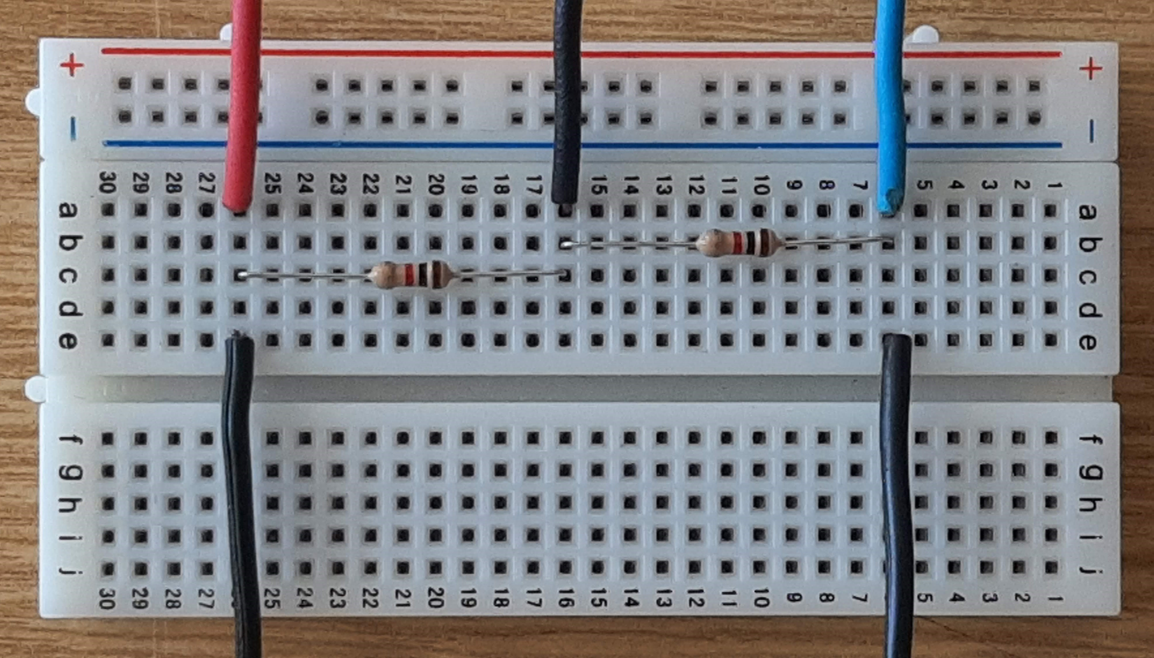
- Constant resistors (in the discipline Electrical Engineering)
 |
| Fig. 11a. Experimental set-up for obtaining the IV curve of a constant resistor 1 k... |
 |
| Fig. 11b. ... in close-up. |
- Variable resistors (in the discipline Electrical Engineering)
 |
| Fig. 12a. Experimental set-up for obtaining the IV curve of a variable resistor 1 k... |
 |
| Fig. 12b. ... close up... |
- photoresistors (in the discipline Semiconductor Devices)
 |
| Fig. 13a. Photoresistor on the board close-up... |
- Thermistors (Semiconductor Devices)
- Conductive foam (Electrical Engineering)
 |
| Fig. 14a. Experimental set-up for obtaining the IV curve of conductive foam. |
 |
| Fig. 14b. ... next to the board, close-up. |
- Graphite resistors (drawn on paper) - Electrical Engineering
- Water (salted) - Electrical engineering"
- Human body - Electrical engineering
- Short circuit (piece of wire) - Electrical engineering
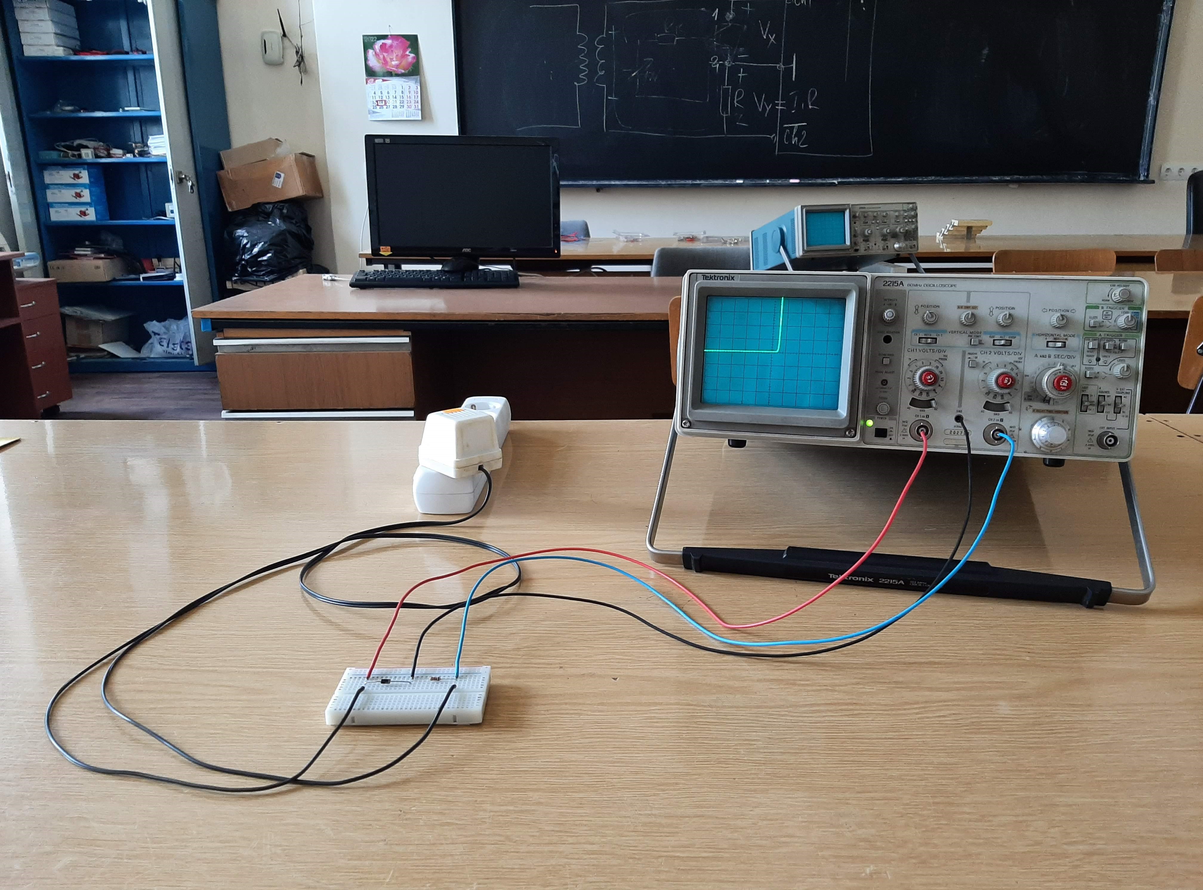
 |
| Fig. 15a. Experimental set-up for obtaining the IV curve of a short circuit (piece of wire) |
 |
| Fig. 15b. ... on the board, close-up. |
 |
| Fig. 15c. IV curve of a short circuit (piece of wire) |
- and open circuit ("nothing") - in "Electrical Engineering"
 |
| Fig. 16a. Experimental set-up for obtaining the IV curve of an open circuit ("nothing":) |
 |
| Fig. 16b. ... and on the board in close-up |
 |
| Fig. 16c. IV curve of an open circuit ("nothing":) |
- Measuring devices of various ranges - Electrical engineering:
 |
| Fig. 17a. Experimental set-up for obtaining the IV curve of a voltmeter |
 |
| Fig. 17b. IV curve of a voltmeter (range 20 V) |
 |
| Fig. 18a. Experimental set-up for obtaining the IV curve of a 2 mA ammeter |
 |
| Fig. 18b. IV curve of an ammeter (range 2 mA) |
- Batteries - Electrical Engineering:
 |
| Fig. 19a. Experimental set-up for obtaining the IV curve of +3 V battery |
 |
| Fig. 19b. IV curve of a battery (+3 V) |
 |
| Fig. 19c. Experimental set-up for obtaining the IV curve of -3 V battery |
 |
Fig. 19d. IV curve of a battery (-3 V)
|
 |
| Fig. 19e. Experimental set-up for obtaining the IV curve of +1.2 V battery in close-up |
 |
Fig. 19f. IV curve of a battery (+1.2 V)
|
 |
| Fig. 19g. Experimental set-up for obtaining the IV curve of -1.2 V battery in close-up |
 |
| Fig. 19h. IV curve of a battery (-1.2 V) |
- Diodes - Semiconductor Devices:
 |
| Fig. 20a. Experimental set-up for obtaining the IV curve of a silicon diode 1N4007 |
 |
| Fig. 20b. 1N4007 silicon diode on the board close-up |
 |
| Fig. 20c. IV curve of a silicon diode 1N4007 |
 |
| Fig. 20d. Experimental set-up for obtaining the IV curve of a germanium diode (a junction of SFT 323) |
 |
| Fig. 20e. Germanium diode (SFT 323 transistor junction) on the board close-up |
 |
| Fig. 20f. IV curve of a germanium diode (SFT 323 transistor junction) |
 |
| Fig. 20g. Experimental set-up for obtaining the IV curve of a 5.1 V Zener diode |
 |
| Fig. 20h. 5.1 V Zener diode on the board close-up |
 |
| Fig. 20i. IV curve of a 5.1 V Zener diode |
- LEDs (in different colors)
 |
| Fig. 20j. Experimental set-up for obtaining the IV curve of a red LED |
 |
| Fig. 20 k. Red LED on the board close-up |
 |
| Fig. 20l. IV curve of a red LED |
Connecting LEDs with different threshold voltages in parallel


Comments
Post a Comment